For Python application developers looking to harness the power of machine learning, understanding the foundational tools is critical. Among those tools is PyTorch, a leading open-source machine learning framework renowned for its flexibility, Pythonic interface, and dynamic approach to computation.

This guide is designed to demystify PyTorch's core components, providing you with a solid understanding of how it empowers the creation and training of sophisticated machine learning models. We'll break down the essentials into three interconnected concepts:

1. Tensors: The fundamental building blocks of data in PyTorch
2. Neural networks: The architectural models that process this data
3. Autograd: PyTorch's powerful engine that enables networks to learn from their experience

By understanding these pillars, you'll gain insight into how PyTorch facilitates the development of intelligent applications, from image classification to complex predictive systems.

What is PyTorch?

PyTorch is a foundational, open-source machine learning framework, primarily distinguished by its Pythonic interface and dynamic computation graphs. Unlike frameworks that build static graphs upfront, PyTorch's "define-by-run" approach constructs the computational graph dynamically as operations are executed, offering unparalleled flexibility for debugging and experimenting with complex or variable neural network architectures. 

At a high level, a computational graph is a way to represent a sequence of calculations as a graph. In this graph, each node represents a mathematical operation (like addition, multiplication, or a more complex function), and the edges (or arrows) represent the data (usually numbers or tensors) that flow between these operations. You can think of it like a flowchart. When you define a neural network and feed data through it, PyTorch internally builds one of these graphs. It records every step taken to get from your input data to the final output. This graph is crucial because it's what allows frameworks like PyTorch to efficiently simulate and train systems like neural networks. 

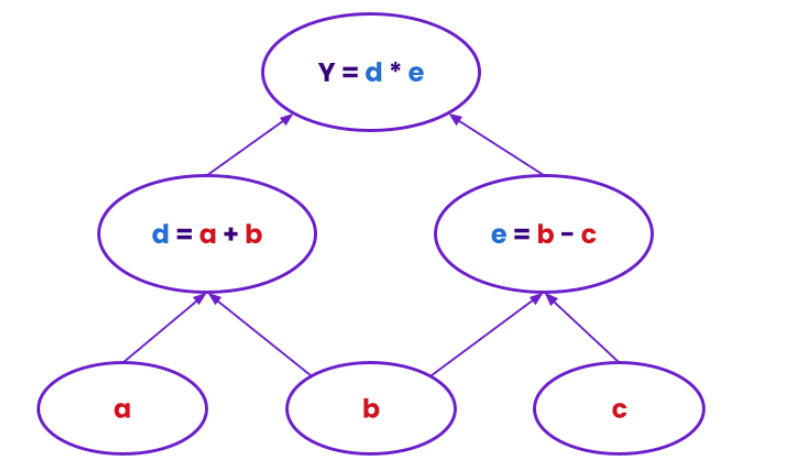
[Caption: An example of a simple computational graph.]

Typical neural network training is done using an algorithm called backpropagation. The idea is to compute the gradient of the error with respect to the parameters used in the network, starting from the end of the network and propagating them to the beginning. PyTorch uses this computational graph to calculate gradients of error during backpropagation. Autograd is a key feature of PyTorch, and it helps automate this process. 

That’s kind of a lot to take in all at once – especially if deep-learning is new to you – so let’s look at tensors, neural networks, and Autograd more in depth.

What are tensors?

Tensors are multi-dimensional arrays (scalars, vectors, matrices, etc.) that hold numerical data. For PyTorch specifically, tensors are the framework’s fundamental data structure upon which everything else is built. If you’ve ever used NumPy `ndarrays`, tensors are like that, except computation can be offloaded to accelerators such as  Graphics Processing Units (GPUs). 

Here is an example of the creation of a tensor in PyTorch.

```

data = [[1, 2],[3, 4]] # Numerical data represented as a 2x2 matrix

x_data = torch.tensor(data) # Converts the 2x2 matrix into a tensor

```

The above code takes a 2x2 matrix of numerical data and converts it to a PyTorch Tensor. The result is a specialized data structure optimized for machine learning. Tensors are used to encode the inputs and outputs of a model, as well as the model’s parameters. All data (images, text, audio, numerical features) you feed into a neural network, and all the intermediate calculations, will be represented as tensors. They are also optimized for automatic differentiation (known as Autograd). Tensors form the building blocks of PyTorch, and almost every operation in PyTorch will act on them. (Refer to the documentation for more information.)

How to represent a neural network in PyTorch?

Inspired by the human brain, an artificial neural network (ANN) is a computational model that processes data through interconnected layers to transform inputs into desired outputs. Each layer is composed of artificial neurons that are connected to neurons in the previous and next layers. Each artificial neuron receives signals from connected neurons, then processes them and sends a signal to other connected neurons. The connection between the neurons is represented by a weight, a numerical value representing the strength of the connection. The signal and the output of each neuron are real numbers. The output is computed by a function of all its inputs and the connection’s strength, called the activation function. These networks learn to perform tasks by adjusting the weights on their internal connections during a training process, allowing them to make accurate inferences and predictions. To illustrate how ANNs learn, let’s look at a simplified example: Classifying images of clothing based on the Fashion-MNIST dataset, which is often used for ML benchmarking. Such a classification model would use images of different articles of clothing to train on to be able to accurately identify a dress as a dress or a sandal as a sandal.

[Caption: A portion of the Fashion-MNIST dataset.]

Let’s build a neural network to do this. One of the most typical and simple neural network is composed of three interconnected layers:

Input layer

This is the layer that consumes the raw input. For a Fashion-MNIST image, each image is typically a 28x28 pixel grayscale image. The input layer would have 784 nodes (28 * 28), with each node receiving the pixel intensity value (e.g., a number between 0 and 255) from one specific pixel in the image. Typically,  each output signal of the neurons will be sent to each neuron of the hidden layer.

Hidden layer

This layer of nodes receives signals from the input layer and processes it further. For a Fashion-MNIST image, a hidden layer might take in groups of pixel values and start to detect rudimentary shapes, edges, or textures (e.g., identifying a vertical line, a curved edge, or a patch of rough texture). If there are multiple hidden layers, a deeper hidden layer might then combine these simpler features to recognize more complex patterns, such as a sleeve, a collar, or the shape of a shoe's sole. There can be many hidden layers, each one a network of nodes further refining and processing the data to extract increasingly abstract features.

Output layer

This layer is responsible for the final result of the processing that has occurred in the hidden layers. In the case of Fashion-MNIST, the goal is to classify the clothing item. Since there are 10 different categories of clothing, the output layer would typically have 10 nodes. Each of these nodes would represent one of the clothing categories, and the network's output would indicate the probability that the input image belongs to each of those categories, depending on the output signals from those 10 nodes (e.g., "95% chance it's a sneaker, 3% chance it's a sandal, 2% chance it's something else").

Neural Network in PyTorch

In PyTorch, `torch.nn.Module` is the foundational base class for all neural networks. You can think of it as an organized container for layers and other modules, defining the complete flow of data through your network. In essence,` torch.nn.Module` serves as the object-oriented blueprint for building neural networks.

So, if we were to build a neural network to classify Fashion-MNIST images, we would inherit from `nn.Module`. In our custom network's`__init__` method, we would set up the specific layers we intend to use. For Fashion-MNIST, this might involve an `nn.Linear` layer to handle the flattened 28x28 pixel input (784 features), followed by `nn.ReLU` for non-linearity, and ultimately another `nn.Linear` for the 10 output classes. Then, in the forward method, we would define the computational sequence, dictating how an input image (represented as a tensor) moves through these layers to produce a classification prediction. PyTorch’s built-in classes and methods for these complex computations mean that you can focus more on architecting and training powerful models rather than implementing the intricate mathematical operations yourself.

Below is an example of how we might do this with PyTorch. This example is derived from the PyTorch documentation, where you can see the details of this implementation.

```

# The following class defines the architecture of the model

class ClothingClassification(nn.Module): # Here is where we use PyTorch’s nn.Module class to inherit from

    def __init__(self):

        super().__init__()

        

        self.flatten = nn.Flatten()

      

        # The following are all different layers that operate on the data in the order they are declared here

        self.linear_relu_stack = nn.Sequential(

            nn.Linear(28*28, 512),

            nn.ReLU(),

            nn.Linear(512, 512),

            nn.ReLU(),

            nn.Linear(512, 10)

        )

    

     # The following defines the computational flow of data as it’s passed

     # from node to node and layer to layer

    def forward(self, x):

        x = self.flatten(x)

        logits = self.linear_relu_stack(x)

        return logits
```

How does the neural network learn, what is Autograd?

Initially, as data flows through the layers of an untrained neural network, the computations result in largely random and incorrect outputs. This is because the network has not yet learned how to accurately process the data. To enable the network to produce correct and expected outputs, we need to teach it by systematically adjusting the mathematical relationships (connection weights for example) within its hidden layers through a process called training. In other words, we need to retrace our steps through our calculations to see where we went wrong.

A common and very powerful algorithm used to train neural networks is backpropagation. This algorithm systematically adjusts the parameters within the network's layers to minimize the difference between its predictions and the correct answers. While backpropagation is essential, performing these intricate calculations by hand for every parameter in a large neural network would be incredibly arduous, tedious, and highly prone to errors. Fortunately, PyTorch provides Autograd  – an automatic differentiation engine that lies at the heart of neural network training.

At a high level, Autograd keeps the dynamic computational graph to compute the function gradient. This graph precisely tracks all the mathematical operations and "steps" taken to reach the output. Because it's generated on the fly, you can even use standard Python control flow like if/else statements and for-loops within your network's logic, but be aware that this is not a good practice. 

When the model produces an incorrect prediction (quantified as the loss function), Autograd enables it to efficiently move backward through this computational graph, from the output layer to the input. Using the gradients computed at each step, each parameter is updated to reduce the loss, effectively teaching the network to make more accurate predictions over time.

Conclusion

AI and ML are formidable new additions to our arsenal of tools. However, as this discussion has highlighted, a deep comprehension of these tools is essential. PyTorch's power is matched by its complexity, creating pitfalls for the unwary developer. To understand PyTorch complexity and writing flawless code, automated enforcement is a must have. In our next blog post, we'll dive into the practical application of this safeguard, exploring specific static analysis rules designed to verify your PyTorch usage, and ensure you're leveraging its power correctly and securely.